Viewing Meta-Heuristic Synchronization using the Path Integral Interpretation

We can investigate and compare the probabilistic representation of the path integral theory with the description of a metaheuristic signalling algorithm as a system of discontinuous pas-coupling.

Discontinuous pas coupling can occur in a variety of system. It is especially important in the field of wireless signalling, such as using radio waves, microwaves or optical light sources such as LEDs and Lasers to transmit data. In such a system, where information packets are transmitted and received, you have quite naturally a discontinuity based on external and internal natures of the transmission infrastructure, interference, decoherence and obstructions.

So lets say we are interested in discontinuous pas coupling, as the strategy to achieve synchronization. Within such a system you might have arbitrary network conditions, individual delays and additionally you will have appropriately to receive packets.

This means that there is a random chance that the signal that is transmitted is not going to be received. This has all to be taken into account and, as discussed in our article on metaheuristics, is when why use metaheuristic algorithms that contain randomization elements along with the nature of the transmission power law function in order to achieve and guarantee synchronization between oscillating nodes.

Let us take our oscillators running on a unit circle in phase-space. The oscillators represented on a circle in phase space. To achieve synchronization, the oscillators runs clockwise on the circle until it passes the threshold. Whenever it passes the threshold, it will emit a signal pulse, with some probability, Psend. When the oscillators are coupled, they will adjust their individual rates, or periods, of signalling to match with one another (encroaching closer together on the unit circle in phase-space) to achieve synchronization under a time evolution.

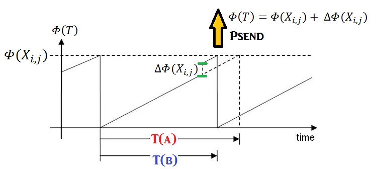
Each oscillator will adjust its period of signalling according to our signalling activation function, which is, under the signalling field representation, a phase function:

The function evolves linear over time, until it reaches a threshold value, defined by the vector weights, X i,j, which are translated into coupling strengths under the powerlaw-based metaheuristic as explained previously.

When the threshold is reached, a single oscillator fires the signal pulse and then resets its phase. If no coupling occurs, the oscillator will pulse with a period, T(A). T is effectively the encoded time remaining until the next signal pulse.

When a phase-coupling occurs between oscillators, when an oscillator receives a pulse it will increment its phase function by an amount that itself depends on its current value and the change induced by the weights of the received signal. The oscillator will then pulse with a new period, T(B):

This means that an oscillator, that is in the lower half of the phase-space circle, will jump forward, and an oscillator that is in the upper half, will jump backwards in the circle in phase space. This is the main concept of a self-organizing update function, which brings the 2 oscillators in phase with one another and thus coupled.

The resemblance of the unitary time-evolution operator in quantum mechanics to the monotonically decreasing signalling function is obvious in their respective mathematical forms:

Moreover, like the unitary time-evolution operator, the signalling algorithm is readily compatible with Lagrangian mechanics in the same way as the unitary time-evolution operator which are inherently used for discrete particles each with a finite number of degrees of freedom.

The classic Lagrangian is written as the difference of the kinetic and potential energy density of a particle.

The potential energy density of the particle is a field density, such as an electromagnetic field density in generalised coordinates V(q).

Since v=p/m, the kinetic energy can of course be written in terms of momentum, p,  which is more relevant for what we are describing.

The abbreviated action S0 is defined as the integral of the generalized momenta along a path in the generalized coordinates q

in our ad-hoc system of synchronization coupling, the momenta will be replaced by Psend and integrated over the time domain (dt) in the path it takes to achieve synchronization. This leads to the total Signalling Action,Sf, being represented as the phase of each path being determined by ∫ Psend dt, for that trajectory.

The frequency of signalling is then, as an oscillation in phase-space:

Using this in the path-integral view we can represent the synchronization procedure as:

In this convention, the signalling action, Sf, which is a real operator is defined as being essentially characteristic of the physical and environmental parameters of the system – namely the light absorption coefficient and the power law over the distance by which it is subject to.

Since each deviation from the path of least action is, just like in the case with a quantum particle, proportional to the action imparted on the system, the signal activation function will activate with a frequency proportional to the action. Therefore, the path of least possible action, which occurs during complete internal synchronization, should have the lowest frequency of signal function activation.

An increase in frequency of signal activation indicates a deviation from the path of least possible signalling action.

Therefore, when using any metaheuristic algorithm, when looking for any deviations, i.e. faults, between the coupled oscillators when internal synchronization is achieved we should just have to look for any changes in the frequency of the signalling between the different nodes.

What do I mean by this?

I mean that when an interaction occurs with our signalling model, the deviation leads to a deviation from the path of least signalling action to achieve synchronization, as we have imparted our own equivalent signalling action, Sf, onto the system.

This causes an initial synchronization collapse. However, the action, Sf, imparted towards the path will lead to an increase in the rate of cycles, i.e. an increase in the signalling action away from the least signalling action, and thus an increase in the probability of achieving synchronization with neighbours again.

In effect, internal processes are stimulated under any signalling action, increasing their state of energy, which is “unfavoured” - unfavoured as the increasing energy state will itself drive the quantised nodes, which have a discrete threshold, that make up the system to spend more energy and thus increase cycling which overall increases the probability that the area under interaction will be synchronized with its neighbours again. Therefore the system is able to restore itself back to synchronization. 

For example, we can have an experimental system of coupled oscillators, as described above, that achieve synchronization through emitting signals to one another over a time series. In the beginning, our 2 (or more) oscillators can be viewed as having similar signals over the time series but are out of phase with each other. As before, the update function is designed to change the period of emitting the signal pulse,(i.e.  T(A) , to T(B))
for each of the oscillators until they achieve synchronicity. In effect we are aligning the time sequences of the 2 signals. 

Dynamical Time Warping, DTW is a technique used for measuring the similarity between two sequences of data in terms of their distances and allowing to find the optimal path to align them in phase. Therefore, it can be a way to represent the degree of coupling between 2 oscillators, signalling in a time series. 

A great many measures of “distance” between 2 different time series of signals have been developed, sometimes called "clustering distances". These are used in many fields involving clusters of data in a signal such as in image analysis, signal processing and machine learning.  

The 3 main types of clustering distances are Euclidean, Manhattan and Minkowski distances:

We shall be using Euclidean Distance as our preferred distance metric, for the simple reason that for our universal power-law signalling algorithm the distance between any 2 nodes is a Euclidean distance using Cartesian coordinates. 

So in the Euclidean distance the sequences are aligned "one-to-one" with the ith point on one time series aligned with the ith point on the other. This itself produces a poor measure of similarity between 2 signals.


In DTW, non-linear alignments (i.e. out of phase sequences T(A) and T(B) ) can be made, thus better measures of similarities between sequences can be made:

In DTW we compare the 2 time series while accounting for the distances, or "warping" (shown above as the coloured lines between T(A) and T(B) ) between the non-linear alignments by dynamic programming. The warp is then resolved by either adding samples or deleting samples.

The warping between the 2 series is calculated by constructing an M x N matrix, which we shall call P.

For P = M x N 

M is the length of one time series: X = X1,...XM

N is the length of the other time series: Y = Y1,...YM

The Euclidean distance is now made up of 2D vectors, Xi and Yj, with each point in the matrix position being p(i,j).

p(0,0) is classified as 0 

p(i,0) and p(0,j) are classified as infinity

The optimum path is calculated by minimizing the degree of warping that occurs in the diagonal paths through this matrix. This is done by comparing, in each matrix cell (i,j),  the time series up to position i in X and position j in Y by the following recursion: 

Which gives us the minimum coordinate distance for each element as: 

By this recursion method we achieve the total warping path, W.

In terms of use in the path integral interpretation of synchronization, the total warping path is equivalent to the total Signalling Action,Sf.

Defining the total warping path, W = W1,...Ws,....Wk. 

The points of the Matrix the warping passes across are 

Ws=(is,js), s=1,2, …,k. 

d(Ws) is an individual distance between corresponding elements of series T(A) and T(B).



The total warping between sequence T(A) and T(B) is therefore:

Which is our DTW recursive function.

To isolate the path of least action, or least warping, some restrictions need to be applied to the recursive function. These include the following:

• Monotonic condition: the path will not turn back on itself, both the i and j indexes either stay the same or increase, they never decrease.
• Continuity condition: the path advances one step at a time. Both i and j can only increase by at most 1 on each step along the path.
• Boundary condition: the path starts at the bottom left and ends at the top right.
• Warping window condition: a good path is unlikely to wander very far from the diagonal. The distance that the path is allowed to wander is the window width. For example, a given warping path, W, should be within the distance between (j = i+W) and (j=i-W)
• Slope constraint condition: The path should not be too steep or too shallow. This prevents short sequences matching too long ones. The condition is expressed as a ratio p/q where p is the number of steps allowed in the same (horizontal or vertical) direction. After p steps in the same direction is not allowed to step further in the same direction before stepping at least q time in the diagonal direction.

In this way the number of possible paths is greatly reduced to only those of particular interest.

In the diagram below we show how DTW give a optimal path (arrangement) to minimize the total distance between the two series, a test series and a reference series. 

The above is a reference set compared against one node. The same is repeated for all the trained ones in the network.

For a particular oscillator (test) in comparison to the rest of the system (reference) the system is 100% synchronized over time when we have a perfect diagonal along the grid generated between the test sample and reference.

By then exposing the synchronized system (i.e. the reference) to a non-synchronized light source, or by introducing a new oscillation, we can induce a deviation from the path of least action of the system that leads to a initial synchronization collapse. This is represented by the path warping in the DTW picture.

However, the collapse, or warp, itself increases the rate at which the disturbed oscillators signal to one another by the metaheuristic procedure, i.e. increases the energy consumption of the system. However this itself in turn increases the probability of restoring synchronization and the state of least energy consumption, least action, possible for the system and so the diagonal path through the grid can be restored.

Constructing Neural Networks from Multiple Synchronized Oscillators

Using this information in our view of meta-heuristics we can go further and incorporate this into neural network structures under the path integral interpretation.

The system of synchronized coupled oscillators forms the neural network structure. We can then reduce the input vectors to an input signalling action oscillating at a certain input frequency in the complex plane,which passes through the network, for example under sigmoidal or other Gaussian analog activation functions, in our path integral interpretation. 

This then gives an output signalling action, or "class", of certain nodes in the network which will now carry a period of oscillation, characteristic of the input signal as interpreted by the neural network. The weights the input vector acts on in the neural network picture are then replaced by the paths in the sum over all possible taken in the time-evolution to achieve synchronization within the network.

I represent this construct in the diagram below, in which I have created a Radial Basis Function synchronized neural network in Matlab which receives a signal and creates an output response characteristic of this input, broadened by the k-number of paths of sigmoidal activation function signalling within the network:

We then say there is an output “class” of internal node signalling action in the network from being stimulated by an external signalling action, in which sense our input signalling action is interpreted as a “class” by the nodes after passing through the neural network.

It is perhaps important to note that the signalling action towards the generation of nodal output classes is clearly not the core function of the neural network and is merely ancillary to it. By this I mean that the vector inputs and their associated weights cause action on the network but in this case are not in fact forming the network structure itself. 

In summary, a network structure can be formed, independently, by the time-evolution of the discontinuous pas-coupling generated by the meta-heuristic nature of the internal signalling which can in principle be described using a path integral interpretation.